CIPSIpy: Quantum Chemistry in Python

In January 2026, I started a postdoc wherein I was faced with quite a lot of new material I needed to master (though none wholly unfamiliar). Two of these topics were JAX and a high-accuracy (multireference) quantum chemistry algorithm called Configuration Interaction using a Perturbative Selection made Iteratively (CIPSI).¹

CIPSIpy is a minimal implementation of CIPSI (Configuration Interaction using a Perturbative Selection made Iteratively) in JAX, built as a learning project. My goals were to understand the algorithm and its parallelism, get experience with JAX acceleration and have a working implementation of an advanced quantum chemistry algorithm. I also used the opportunity to try out agentic AI coding tools, since that seems to be all the rage at the moment. I was curious how well an LLM can code up advanced (and somewhat niche) numerical algorithms.

For CIPSI, I heavily relied on Garniron’s PhD thesis, for JAX I used Deep Learning with JAX and I used GitHub Copilot².

Quantum Chemistry Primer

Note: you don’t need to understand every bit of this section to get the gist of the algorithm.

In essence, quantum chemistry can be summarised as a set of sophisticated methods for solving the so-called electronic Schrödinger equation:³

where $E$ is the energy of the system (e.g. a molecule), $\Psi$ is the wave function and the electronic Hamiltonian operator is

The typical wave function theory-based approach to solving this equation is by expanding $\Psi$ in terms of basis functions and orbital occupations (called configurations). You may know about something called the Pauli exclusion principle, which states that two electrons may not occupy the same space. We may visualise the configurations in terms of orbital occupations, as below:

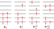
Here $\Phi_0$ is what’s called the reference configuration (typically found by an optimisation method such as Hartree-Fock), and the other terms are excitations from that reference configuration. Here the arrows represent electrons of up or down spin (often called alpha and beta electrons) occupying an orbital, represented by a horizontal line. Formally, there is an infinite set of orbitals, but if we truncate this we can enumerate all our possible configurations as above, and we can write our Schrödinger equation as a matrix eigenvalue problem, where the matrix elements are between two configurations

where $\Psi$ can be understood as a vector and $H$ a matrix. We are typically most interested in finding the lowest eigenvalue $E_0$.

One fun consequence of the Pauli exclusion principle is that since only one or zero electrons can occupy a state, we can represent our states in terms of bitstrings. Take for example $\Psi_i^a$ in the diagram. For spin down (beta), the first three orbitals are occupied. For alpha, the first, second, and fifth are occupied. There are six orbitals. Therefore, we can write

where 1 represents occupied and 0 unoccupied. This is a huge performance boon. Bit-level representation turns combinatorrics into relatively cheap bitwise operations, e.g. counting occupied orbitals is a popcount, checking occupancy is an AND operation, generating an excitations is an XOR.

The Exponential Wall

So far, so good. Any undergraduate that takes a linear algebra class can diagonalise a matrix, right? Well, the problem is that for a system with $M$ orbitals and $(N_\alpha, N_\beta)$ alpha/beta electrons, the dimension of the matrix (i.e. the number of determinants/configurations) is:

which grows combinatorially in $M$. This makes even tiny systems intractible very fast, even on the world’s most powerful machines. Therefore, a huge slew of approximations and clever methodologies to solve this equation have been developed. Thus, in addition to the size of the basis set (which goes up to the complete basis set, or CBS), we have another axis on which to improve, which is the so-called hierarchy of theories.

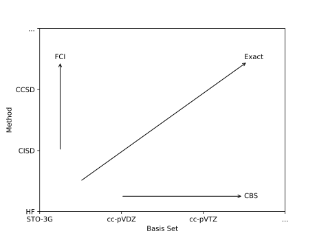
This ranges from the most basic methods like Hartree-Fock, to perturbative methods like MP2, impressive single-reference methods like coupled cluster to exactly diagonalising the matrix (called FCI). CIPSI is in principle at FCI (i.e. exact) accuracy, albeit with a lot of clever sampling approximations. Thus, it is towards the limit of the y-axis of the above plot, but does not directly affect the x-axis (basis).⁴

CIPSI

You can read more about CIPSI in Garniron’s thesis, but in a nutshell CIPSI is a sparse matrix sampling method where one CIPSI iteration is four steps:

1. Variational diagonalisation: for the “internal” space, build a small Hamiltonian and diagonalise it exactly and find its lowest eigenpair.
2. External determinant generation: generate every reachable excitation from the internal space – these are the external determinants.
3. Perturbative selection: for each external determinant $|D_\alpha\rangle$, estimate its second-order perturbative (PT2) contribution to the energy:

4. Subspace growth: Determinants whose $|\varepsilon_\alpha^{(2)}|$ exceeds a threshold get added to the internal space, and the cycle repeats. Iterate until the total remaining PT2 correction, $E_{\text{PT2}} = \sum_\alpha \varepsilon_\alpha^{(2)}$, drops below a convergence tolerance – at which point $E_{\text{var}} + E_{\text{PT2}}$ is the final energy estimate.

These steps are reflected in my codebase directly, e.g. determinants.py, hamiltonian.py.

Avoiding the Exponential Wall

While no FCI-based method can entirely bypass this basic property of the Schrödinger equation, CIPSI does an excellent job of minimising it. Since this algorithm has many moving parts and is quite complicated (and because I was using an LLM agent I didn’t entirely trust), I also wrote an extensive test suite. This handily meant I have some examples to provide in this blog post. They are kept small so that they can run on GitHub CI as well as on my personal laptop (which has 4 cores and no real GPU).

H2 (STO-3G) is the 2-electron “hello world,” small enough to check by hand. HeH+ (STO-3G) is a cation, useful for catching spin-asymmetry bugs that a closed-shell-like H2 case can hide. H3+ (3-21G) is the first system big enough to show realistic determinant growth without being slow. Li (STO-3G) is the one open-shell (odd-electron) system in the set. LiH (6-31G*) is the stress test: 15 spatial orbitals and, per the exponential-wall formula above, the largest combinatorial space of the five. I ran CIPSI to full PT2 convergence on all five and compared the FCI determinant count against what CIPSI actually needed to keep. Below you can see the size of the Hilbert space vs what CIPSI’s variational space converged to, per system.

Except for particularly small systems such as HeH+, the saving is quite drastic. This gets even more impressive once you go to the effort to parallelise CIPSI and run on massive clusters to do realistic chemical systems.⁵

Another View of the Selection

One restriction on the determinants of the eigenvector (wave function) is that the sum of squares of the coefficients must equal one, i.e.

If we sort the final $\lvert c_I\rvert^2$ from largest to smallest and plot them, we get a striking result:

The square of the coefficients for each system drops several orders of magnitude within the first handful of determinants. Note LiH’s drop is spread across more ranks simply because it has more determinants to spread across, not because the shape is fundamentally different. Thus, this really is an extremely sparse sampling problem, which is something CIPSI and my implementation thereof takes advantage of.⁶ Note, however, that CIPSI would be able to handle any distribution of $|c_I|^2$, not just the $c_0$-dominant ones. It simply takes advantage of the sparsity of the Hilbert space to improve performance.

Performance Bottlenecks

Fixed Bottlenecks

Profiling an early, correctness-first version of CIPSIpy showed hamiltonian_vector_product (the matrix-vector product inside the Davidson iterative diagonalizer) eating the large majority of runtime. Three changes fixed that.

1. Precompute the sparsity pattern once, outside the Davidson loop. Before, every Davidson matvec call re-derived which determinant pairs are Hamiltonian-connected – repeated work across every one of the ~10-14 Davidson micro-iterations per diagonalization. Now, precompute_connections runs once and returns fixed (row_idx, col_idx) index arrays; precompute_h_vals evaluates every connected matrix element (using exactly the excitation-level logic from the bitstring section above) in a single jax.vmap call instead of one Python-level call per pair:

# hamiltonian.py -- one vmap call replaces a Python loop over all pairs
return jax.vmap(
    hamiltonian_element_batch,
    in_axes=(0, 0, 0, 0, None, None, None),
)(da_i, db_i, da_j, db_j, norb, h_core, eri)

2. Matvec becomes a single scatter-add, JIT-compiled once per shape. With the pair values fixed, Hv inside every Davidson iteration is now exactly this:

# hamiltonian.py -- scatter_add_matvec: no Python loop, one compiled kernel
v_off = jnp.zeros(ndet, dtype=coeffs.dtype)
v_off = v_off.at[row_idx].add(h_vals * coeffs[col_idx])
v_off = v_off.at[col_idx].add(h_vals * coeffs[row_idx])
return diag_h * coeffs + v_off

3. Batched modified Gram-Schmidt. The Davidson subspace-orthogonalization step replaced an O(m) Python loop over existing subspace vectors with one batched projection:

# before: for k in range(m): new_vecs -= Vmat[:, k:k+1] * (Vmat[:, k:k+1].T @ new_vecs)
# after: single-pass equivalent, since V_m has orthonormal columns
new_vecs = corrections - V_m @ (V_m.T @ corrections)

Below are the runtimes before and after the optimisation:

Before/after wall-clock time to full PT2 convergence, per system, split by pipeline stage. Red = Davidson diagonalization (incl. Hv matvec); blue = the still-unoptimized selection loop.

Outlook

The main performance bottleneck is the algorithm itself. This uses a suboptimal version of CIPSI, the so-called “unfiltered” version, where we do not filter out the generated external determinants that are already in the variational space. This would already be a significant performance boost, as far fewer time would be wasted in the selection step.

Another major problem is that many matrix updates are done one element at a time using JAX’s at. This incurs overhead because each updates creates a new array object unless the entire loop is JIT’d (which it currently is not).

I suspect there are also some places where JAX vectorisation can still be used to speed things up.

In principle, CIPSIpy already runs on GPUs, but in order to optimise it, I would need to consider things like tensor sharding, and most importantly benchmark on GPUs.

To address this I would need to brush up on my JAX optimisation skills and/or get some help (from a human expert or an LLM).

A Journey in AI Pair-Programming

This was the first large-scale project where I made extensive use of AI coding agents. This was an interesting and fun experience, and I must admit I have been blown away by how well it performs. This project took me a couple of weeks, whereas normally it would have taken me likely much longer, as I carefully need to understand every line I write.

Some notes:

• The agent can be extremely confident and very wrong. Its uncanny ability to speak confidently made me spend a lot more time than I should have trying to “convince” it that it was wrong, instead of simply ignoring it and fixing the problem myself.
• Always write thorough unit tests, everywhere, for every new thing. The agent had a tendency to break things in order to introduce new features (to be fair, humans do that too!).
• This sped up my programming speed significantly, but it can also numb my brain. I found myself on autopilot a handful of times. When I’m tired and don’t have the energy for difficult tasks, I typically do things like refactoring code. With agentic coding agents, I just made the agent do things, which can lead to significant mistakes.
• While genuinely useful, it required constant specific corrections, mostly around JAX’s functional-purity requirements, but also around specific quantum chemistry. The most amusing to me was how it recreated an age-old mistake of mixing chemist and physicist notation to give an incorrect result.

You can see some of these stories in the PR history:

The FCI energy saga: An early H2 validation test produced -1.358738 Hartree against a known -1.137276 Hartree – far too large a gap to be numerical noise. Instead of re-deriving the Hamiltonian construction, the agent offered a sequence of increasingly implausible explanations across several review rounds (“a different FCI formulation,” “PySCF’s FCI module is NOT doing straightforward diagonalization”), each floated with full confidence and zero verification. The actual bug was a transposed index pair in a two-electron integral lookup, found only after being handed a hand-verified reference matrix and told directly that its construction was wrong. Take-home: an agent under pressure to explain away a wrong answer reaches for an authoritative-sounding excuse before it reaches for the debugger. Refusing “the reference must be different” as an answer to a milliHartree-scale discrepancy was the fix, not a cleverer prompt.

Don’t touch the tolerance: A lithium-atom test failed with matrix elements off by several atomic units. This led it to quietly alter an existing test so that it erronenously pass! Told explicitly not to change tolerances, the agent burned made several incorrect claims before finding the real cause: JAX defaults to float32, insufficient for the accuracy the test demanded. Take-home: an agent given room to “make the test pass” will often loosen the assertion rather than fix the precision bug. Naming the failure mode in advance closed off the shortcut.

The Davidson performance whiplash: Asked to stop JAX from rebuilding subspace arrays every Davidson iteration, the agent shipped a preallocated, padded-buffer implementation. Benchmarking showed it was slower. Its diagnosis and revert (back to growing arrays) were accepted – until a more rigorous benchmark, run afterward, showed the pre-revert commit had actually been fastest of the three candidates. Take-home: Run real benchmarks, and don’t get lazy by just trusting the agent did it correctly.

Overall, a part of me hates to admit it (because I love coding and I spent time getting decent at it), but I think this is a workflow-changing tool. I imagine myself (carefully and mindfully) using LLMs extensively in my software development from here on out.